Note
Click here to download the full example code
Adding an inset to the figure
To plot an inset figure inside another larger figure, we can use the
pygmt.Figure.inset method. After a large figure has been created,
call inset using a with statement, and new plot elements will be
added to the inset figure instead of the larger figure.
import pygmt
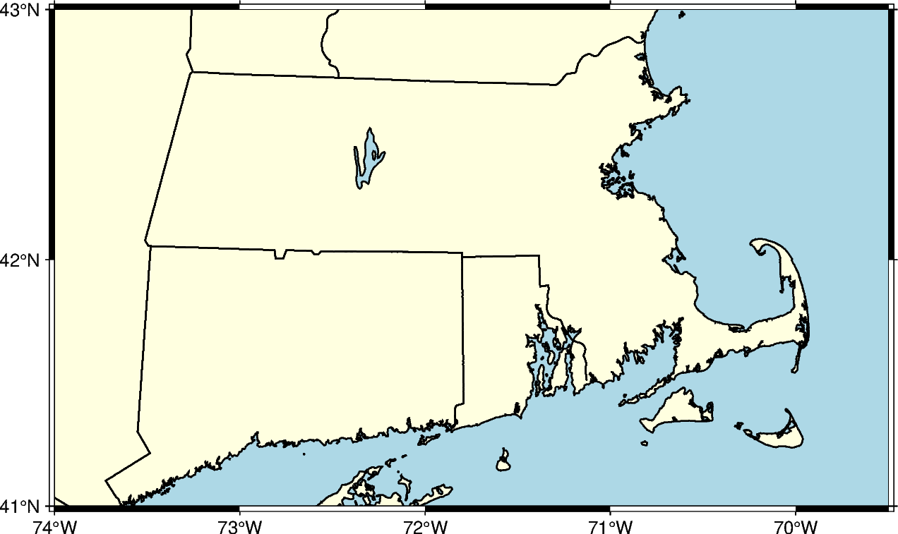
Prior to creating an inset figure, a larger figure must first be plotted. In the
example below, pygmt.Figure.coast is used to create a map of the US state of
Massachusetts.
fig = pygmt.Figure()
fig.coast(
    region=[-74, -69.5, 41, 43],  # Set bounding box of the large figure
    borders="2/thin",  # Plot state boundaries with thin lines
    shorelines="thin",  # Plot coastline with thin lines
    projection="M15c",  # Set Mercator projection and size of 15 centimeter
    land="lightyellow",  # Color land areas light yellow
    water="lightblue",  # Color water areas light blue
    frame="a",  # Set frame with annotation and major tick spacing
)
fig.show()
Out:
<IPython.core.display.Image object>
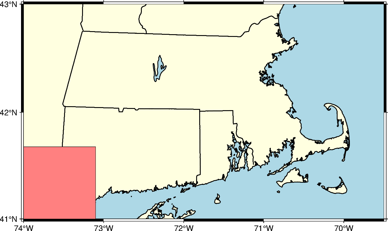
The pygmt.Figure.inset method uses a context manager, and is called using a
with statement. The position parameter, including the inset width, is
required to plot the inset. Using the j argument, the location of the inset is
set to one of the 9 anchors (bottom-middle-top and left-center-right). In the
example below, BL sets the inset to the bottom left. The box parameter can
set the fill and border of the inset. In the example below, +pblack sets the
border color to black and +gred sets the fill to red.
fig = pygmt.Figure()
fig.coast(
    region=[-74, -69.5, 41, 43],
    borders="2/thin",
    shorelines="thin",
    projection="M15c",
    land="lightyellow",
    water="lightblue",
    frame="a",
)
with fig.inset(position="jBL+w3c", box="+pblack+glightred"):
    # pass is used to exit the with statement as no plotting functions are called
    pass
fig.show()
Out:
<IPython.core.display.Image object>
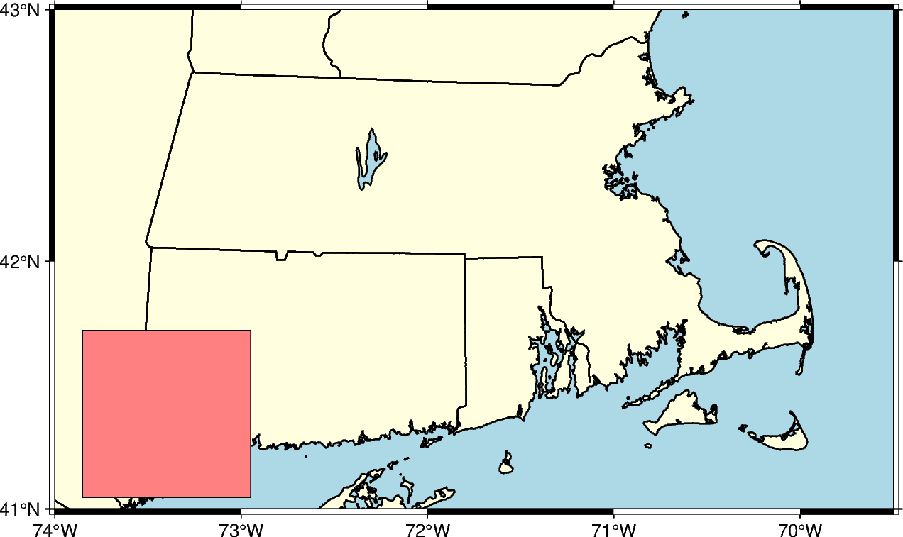
When using j to set the anchor of the inset, the default location is in contact with the nearby axis or axes. The offset of the inset can be set with +o, followed by the offsets along the x- and y-axis. If only one offset is passed, it is applied to both axes. Each offset can have its own unit. In the example below, the inset is shifted 0.5 centimeters on the x-axis and 0.2 centimeters on the y-axis.
fig = pygmt.Figure()
fig.coast(
    region=[-74, -69.5, 41, 43],
    borders="2/thin",
    shorelines="thin",
    projection="M15c",
    land="lightyellow",
    water="lightblue",
    frame="a",
)
with fig.inset(position="jBL+w3c+o0.5c/0.2c", box="+pblack+glightred"):
    pass
fig.show()
Out:
<IPython.core.display.Image object>
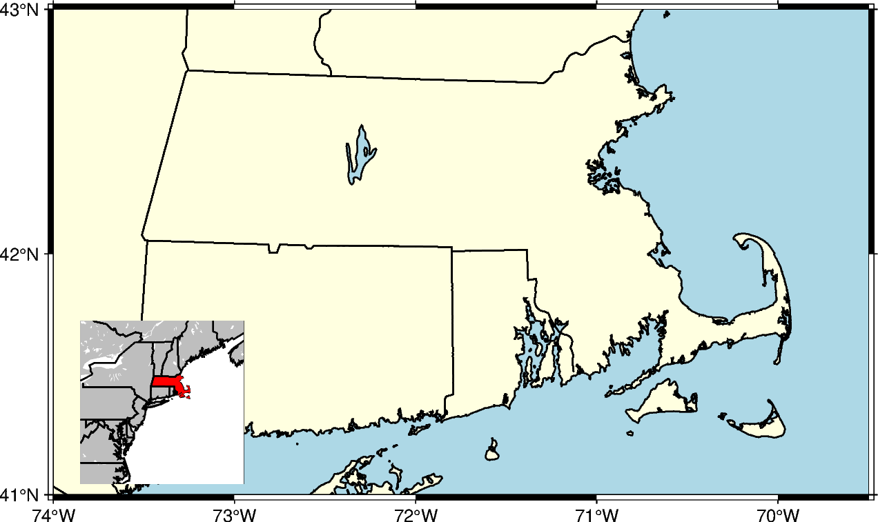
Standard plotting functions can be called from within the inset context manager.
The example below uses pygmt.Figure.coast to plot a zoomed out map that
selectively paints the state of Massachusetts to shows its location relative to
other states.
fig = pygmt.Figure()
fig.coast(
    region=[-74, -69.5, 41, 43],
    borders="2/thin",
    shorelines="thin",
    projection="M15c",
    land="lightyellow",
    water="lightblue",
    frame="a",
)
# This does not include an inset fill as it is covered by the inset figure
with fig.inset(position="jBL+w3c+o0.5c/0.2c", box="+pblack"):
    # Use a plotting function to create a figure inside the inset
    fig.coast(
        region=[-80, -65, 35, 50],
        projection="M3c",
        land="gray",
        borders=[1, 2],
        shorelines="1/thin",
        water="white",
        # Use dcw to selectively highlight an area
        dcw="US.MA+gred",
    )
fig.show()
Out:
<IPython.core.display.Image object>
Total running time of the script: ( 0 minutes 5.847 seconds)